在进行时间序列分析之际,意外之数——异常值,往往会成为其中引人困扰之处。此类异常值犹如数据集中的“刺头”,其出现往往使预测模型偏于预期,使得预估结果产生偏差。试想若因少数异常值致预测失败,岂非遗憾?因此,本文将探讨如何祛除这些异常值,以期提升时间序列分析的精确度。
异常值的危害:不仅仅是“小打小闹”
别小看异常值,对时间序列分析,它们不仅是“小打小闹”,更是数据集内的“癌症”,未能有效清除,可能会严重侵蚀模型的可靠性。曾有案例证明,排除异常值后,模型的平均绝对误差(MAE)精确度明显提高达到了0.1%,这不是一个无足轻重的数字,可见其对模型影响之大。
异常值处理的重要性:不仅仅是“锦上添花”
处理时间序列异常对于分析至关重要,而非“添枝加叶”,实为“雪中送炭”。
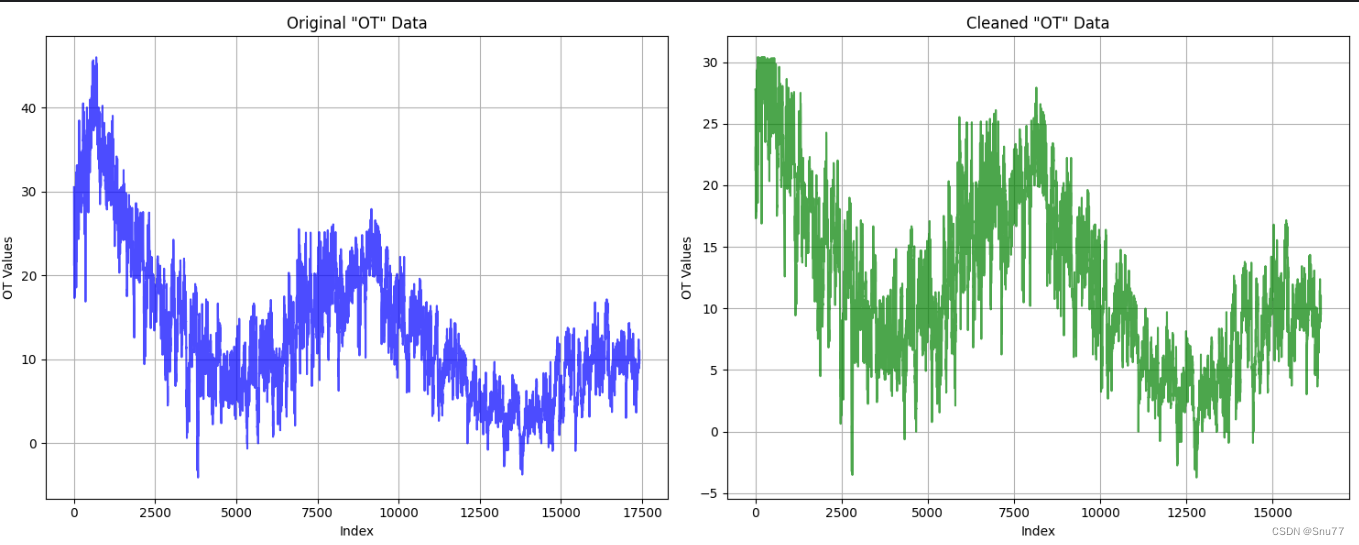
异常值处理的常用方法:不仅仅是“一招鲜”
import pandas as pd
from scipy.stats import zscore
import matplotlib.pyplot as plt
# Load the data
file_path = 'ETTh1.csv'  # Replace with your file path
data = pd.read_csv(file_path)
# Calculate Z-Scores for the 'OT' column
data['OT_ZScore'] = zscore(data['OT'])
# Filter out rows where the Z-Score is greater than 2
outliers_removed = data[data['OT_ZScore'].abs() <= 2]
# Creating a figure with two subplots
fig, axes = plt.subplots(nrows=1, ncols=2, figsize=(15, 6))
# Plotting the original data in the first subplot
axes[0].plot(data['OT'], label='Original Data', color='blue', alpha=0.7)
axes[0].set_title('Original "OT" Data')
axes[0].set_xlabel('Index')
axes[0].set_ylabel('OT Values')
axes[0].grid(True)
# Plotting the cleaned data in the second subplot
axes[1].plot(outliers_removed['OT'].reset_index(drop=True), label='Data After Removing Outliers', color='green', alpha=0.7)
axes[1].set_title('Cleaned "OT" Data')
axes[1].set_xlabel('Index')
axes[1].set_ylabel('OT Values')
axes[1].grid(True)
# Adjusting layout and displaying the plot
plt.tight_layout()
plt.show()
在应对异常数据的问题上,多种技术手段可供选择。譬如利用机器学习建立模型进行预测及替换异常值,具有较高的技术含量和实用价值;此外,也可采用均值替代、中位数取代以及众数置换等方式,但需根据具体情况和需求选择最适宜的方案。因此,如何选择合适的方法,关键在于对异常值特性及其分析目的的深入理解与把握。
平均值替换:不仅仅是“保守”
平均值置换看似保守,实则在处理极端值(即异常值)方面具有显著优势。通过将整组数据的均值置换为异常值,能够降低此类数值对模型性能的干扰,实现模型稳定性提升。不过,该法在数据呈现非对称分布时可能表现稍差。
import pandas as pd
from scipy.stats import zscore
import matplotlib.pyplot as plt
# Load the data
file_path = 'ETTh1.csv'  # Replace with your file path
data = pd.read_csv(file_path)
# Calculate Z-Scores for the 'OT' column
data['OT_ZScore'] = zscore(data['OT'])
# Filter out rows where the Z-Score is greater than 2
outliers_removed = data[data['OT_ZScore'].abs() <= 2]
# Creating a figure with two subplots
fig, axes = plt.subplots(nrows=1, ncols=2, figsize=(15, 6))
# Plotting the original data in the first subplot
axes[0].plot(data['OT'], label='Original Data', color='blue', alpha=0.7)
axes[0].set_title('Original "OT" Data')
axes[0].set_xlabel('Index')
axes[0].set_ylabel('OT Values')
axes[0].grid(True)
# Plotting the cleaned data in the second subplot
axes[1].plot(outliers_removed['OT'].reset_index(drop=True), label='Mean Value Replacement', color='green', alpha=0.7)
axes[1].set_title('Cleaned "OT" Data')
axes[1].set_xlabel('Index')
axes[1].set_ylabel('OT Values')
axes[1].grid(True)
# Adjusting layout and displaying the plot
plt.tight_layout()
plt.show()
中位数替换:不仅仅是“中庸”
中位替换,也被称为中庸法,系利用中位数代替离群值以降低其对模型稳定性的影响。此种方法尤其适合于数据非对称分布的情境,因可显著减轻异常值对模型的干扰。
众数替换:不仅仅是“随大流”
import pandas as pd
from scipy.stats import zscore
import matplotlib.pyplot as plt
# Load the data
file_path = 'ETTh1.csv'  # Replace with your file path
data = pd.read_csv(file_path)
# Calculate Z-Scores for the 'OT' column
data['OT_ZScore'] = zscore(data['OT'])
# Filter out rows where the Z-Score is greater than 2
outliers_removed = data[data['OT_ZScore'].abs() <= 2]
# Creating a figure with two subplots
fig, axes = plt.subplots(nrows=1, ncols=2, figsize=(15, 6))
# Plotting the original data in the first subplot
axes[0].plot(data['OT'], label='Original Data', color='blue', alpha=0.7)
axes[0].set_title('Original "OT" Data')
axes[0].set_xlabel('Index')
axes[0].set_ylabel('OT Values')
axes[0].grid(True)
# Plotting the cleaned data in the second subplot
axes[1].plot(outliers_removed['OT'].reset_index(drop=True), label='Median Value Replacement', color='green', alpha=0.7)
axes[1].set_title('Cleaned "OT" Data')
axes[1].set_xlabel('Index')
axes[1].set_ylabel('OT Values')
axes[1].grid(True)
# Adjusting layout and displaying the plot
plt.tight_layout()
plt.show()
众数置换,即排除异常值后采用众数填充,此法能显著减轻其对模型稳定性的负面影响。然而,这一方法在负值数据情况下表现可能不尽如人意。
分箱法:不仅仅是“简单粗暴”
“分箱法”看似简易明了,实则高效实用。它将数据划分为若干个区间(箱子),再以边界值或中位数等手段替代异常值,从而显著降低异常值对模型稳定性的干扰。该方法在数据分布不平滑的情况下尤为奏效,能有效规避异常值对模型的负面效应。
import pandas as pd
from scipy.stats import zscore
import matplotlib.pyplot as plt
# Load the data
file_path = 'ETTh1.csv'  # Replace with your file path
data = pd.read_csv(file_path)
# Calculate Z-Scores for the 'OT' column
data['OT_ZScore'] = zscore(data['OT'])
# Filter out rows where the Z-Score is greater than 2
outliers_removed = data[data['OT_ZScore'].abs() <= 2]
# Creating a figure with two subplots
fig, axes = plt.subplots(nrows=1, ncols=2, figsize=(15, 6))
# Plotting the original data in the first subplot
axes[0].plot(data['OT'], label='Original Data', color='blue', alpha=0.7)
axes[0].set_title('Original "OT" Data')
axes[0].set_xlabel('Index')
axes[0].set_ylabel('OT Values')
axes[0].grid(True)
# Plotting the cleaned data in the second subplot
axes[1].plot(outliers_removed['OT'].reset_index(drop=True), label='Mode Value Replacement', color='green', alpha=0.7)
axes[1].set_title('Cleaned "OT" Data')
axes[1].set_xlabel('Index')
axes[1].set_ylabel('OT Values')
axes[1].grid(True)
# Adjusting layout and displaying the plot
plt.tight_layout()
plt.show()
手动修改:不仅仅是“费时费力”
在手动修正过程中,是否会感到耗时又费劲呢?其实,这不仅能更精确地处理异常数据,还能使模型更为稳定。
总结:不仅仅是“画龙点睛”
import pandas as pd
import numpy as np
import matplotlib.pyplot as plt
from scipy.stats import zscore
# Load the data
file_path = 'your_file_path_here.csv'  # Replace with your file path
data = pd.read_csv(file_path)
# Calculate Z-Scores for the 'OT' column
data['OT_ZScore'] = zscore(data['OT'])
# Setting a default window size for rolling mean
window_size = 5
# Calculate the rolling mean
rolling_mean = data['OT'].rolling(window=window_size, center=True).mean()
# Replace outliers (Z-Score > 2) with the rolling mean
data['OT_RollingMean'] = data.apply(lambda row: rolling_mean[row.name] if abs(row['OT_ZScore']) > 2 else row['OT'], axis=1)
# Creating a figure with two subplots
fig, axes = plt.subplots(nrows=1, ncols=2, figsize=(15, 6))
# Plotting the original data in the first subplot
axes[0].plot(data['OT'], label='Original Data', color='blue', alpha=0.7)
axes[0].set_title('Original "OT" Data')
axes[0].set_xlabel('Index')
axes[0].set_ylabel('OT Values')
axes[0].grid(True)
# Plotting the data after replacing outliers with rolling mean in the second subplot
axes[1].plot(data['OT_RollingMean'], label='Data After Rolling Mean Replacement', color='green', alpha=0.7)
axes[1].set_title('Data After Rolling Mean Replacement of Outliers')
axes[1].set_xlabel('Index')
axes[1].set_ylabel('OT Values')
axes[1].grid(True)
# Adjusting layout and displaying the plot
plt.tight_layout()
plt.show()
各类方法皆有其特定应用场景及优势劣势。关键在于理清异常值来源及其对分析成果之潜在影响,以确保适当处理。探讨至此,请教各位同仁:贵公司时间序列分析时,又是怎样应对异常值的呢?请于评论区畅所欲言,切勿忘点赞与分享!